Principal components regression analysis for plant physiologists

principal components regression analysis for plant physiologists

Author: Dr. Michael A. Forster

Director, Edaphic Scientific Pty Ltd

It is a common practice for plant physiologists to correlate sap flow, dendrometer or canopy temperature data with environmental variables such as vapour pressure deficit (VPD) or solar radiation. A multiple linear regression model is usually used to determine which environmental variable provides the greatest explanatory or predictive power over the response variable.

A problem with this approach is the issue of collinearity. That is, statistical errors can be introduced into a multiple linear regression model if many of the explanatory variables covary. For example, solar radiation, temperature, relative humidity and VPD usually increase and decrease together throughout a diel (24-hour) cycle.

A statistical method, known as principal components regression (PCR) analysis, has been proposed to resolve the problem of collinearity. PCR is a combination of two statistical methods: principal components analysis (PCA) and multiple linear regression.

The PCA removes the problem of collinearity by creating a series of unrelated components. These components are then used in a subsequent multiple linear regression model to determine their explanatory power over a response variable such as sap flow, dendrometer or canopy temperature data. Different types of multiple linear regression models, for example stepwise, partial, etc, can be deployed to determine which components provides the greatest explanatory power over the variation in the response variable.

This article will highlight:

- a step-by-step guide to performing a PCR analysis;

- the advantages and limitations of PCR;

- the importance of data meeting the assumptions of a normal distribution;

- standardization or translation of data to a common scale;

- presentation of results from a PCR analysis; and

- references and links to programs including R.

a step-by-step guide to PCR

This is a brief overview of how to perform a PCR analysis. Further details on each step are given below.

1) select response and explanatory variables that are relevant;

2) choose timescale for analysis (e.g. 15 minutes, hourly, daily, etc);

3) ensure each explanatory variable is normally distributed or transform data if necessary;

4) standardize or translate each explanatory variable to a common scale;

5) perform a PCA on explanatory variables;

6) extract biologically and physiologically relevant components from the PCA;

7) perform a multiple linear regression analysis with sap flow, dendrometer or canopy temperature data as the response variable and the extracted components from the PCA as the explanatory variables; and

8) present results in table or figure format.

PCR: advantages and limitations

A PCR analysis has two significant advantages:

- PCR eliminates the issue of collinearity; and

- PCR reduces many explanatory variables to fewer explanatory variables.

Although a PCR analysis is a powerful method to analyse a multivariate dataset, as with any statistical method caution needs to be exercised over its implementation and to ensure it assumptions are not violated. Some statisticians argue that there are several failings in the PCR method which must also be considered including:

- choosing which components to retain from the PCA analysis in the multiple linear regression model is often arbitrary;

- variables may be weighted disproportionally to their true importance with insignificant variables given significant importance and vice-versa;

- the most important explanatory variables may be considered equally with “nuisance variables”; and

- explanatory variables may be given the wrong sign such that a negative correlation may in fact be a positive correlation.

Consequently, it is important to carefully consider the results of a PCR and whether it is biologically and physiologically meaningful. A result that defies logic or reason probably indicates an error in the PCR model rather than a novel physiological process!

It is also important to note that PCR is deployed across many scientific disciplines. Many of the limitations, or criticisms, of PCR occur when there are numerous explanatory variables in a model. In some cases, there may be dozens to hundreds of explanatory variables. However, for plant physiologists analysing sap flow, dendrometer or canopy temperature data, usually, there are only a few, albeit highly collinear, explanatory variables to consider. The interpretation and consideration of results is far easier with fewer explanatory variables. A researcher may even consider removing explanatory variables from the analysis that clearly add little value to the analysis or interpretation of results.

timescales of the data for analyses

A plant physiologist often must deal with large temporal datasets. It can be difficult to determine what is a data point. For example, data may be recorded every 15 minutes. Therefore, is this a data point? Or do you take hourly averages? Or daily sums, maximums, averages, etc?

Meeting the assumption of normality is critical for multiple linear regression analysis. This is extremely difficult when there are large datasets such as data recorded every 15 minutes. Summing, averaging or binning large datasets is an acceptable approach to meet the assumptions of normality.

If such manipulations of the data are unacceptable, or may somehow violate hypothesis testing, then alternative statistical methods to a multiple linear regression model should be considered.

normality and the assumptions of PCA

A PCR must meet all the same assumptions as a standard PCA. Importantly, this includes that each explanatory variable must follow a normal distribution. If data are non-normal, then transformations of the data are required such as a log transformation. Other assumptions include (Quinn and Keough, 2002):

- there are linear, rather than non-linear, relationships between explanatory variables (ensuring data meet a normal distribution will assist with this assumption);

- outliers can influence outcomes from a PCA. Removing or dealing with outliers can be difficult; and

- missing data can be a problem. Usually, entire objects, or rows, are removed from an analysis if there is a missing datum.

standardization or translation of data

Environmental variables are usually measured on different scales. For example, solar radiation is measured on a different scale to ambient air temperature which are both measured differently to volumetric soil water content. Transformation of data, such as log transformation, also alters scaling of data.

Prior to entering data into a PCA, it is often recommended to standardize data to the same scale. This process is also known as data translation (Legendre and Legendre, 1998). A common approach is to centre the data so that it has a mean of zero and standard deviation of one (Quinn and Keough, 2002).

presentation of results from a PCR analysis

A PCR analysis is a combination of PCA and multiple linear regression. Therefore, results are typically presented in a similar fashion to a traditional PCA or multiple linear regression analysis.

For PCA, it is common to present the ordination or scaling plot based on the correlation matrix. Usually, component 1 is presented on the x-axis and component 2 on the y-axis. Additional components may also be presented in different figures. For example, Van der Werf et al (2005) presented the relationship between plant species composition and the effects of locusts, grazing, soils and elevation on plant species composition in a ordination plot:

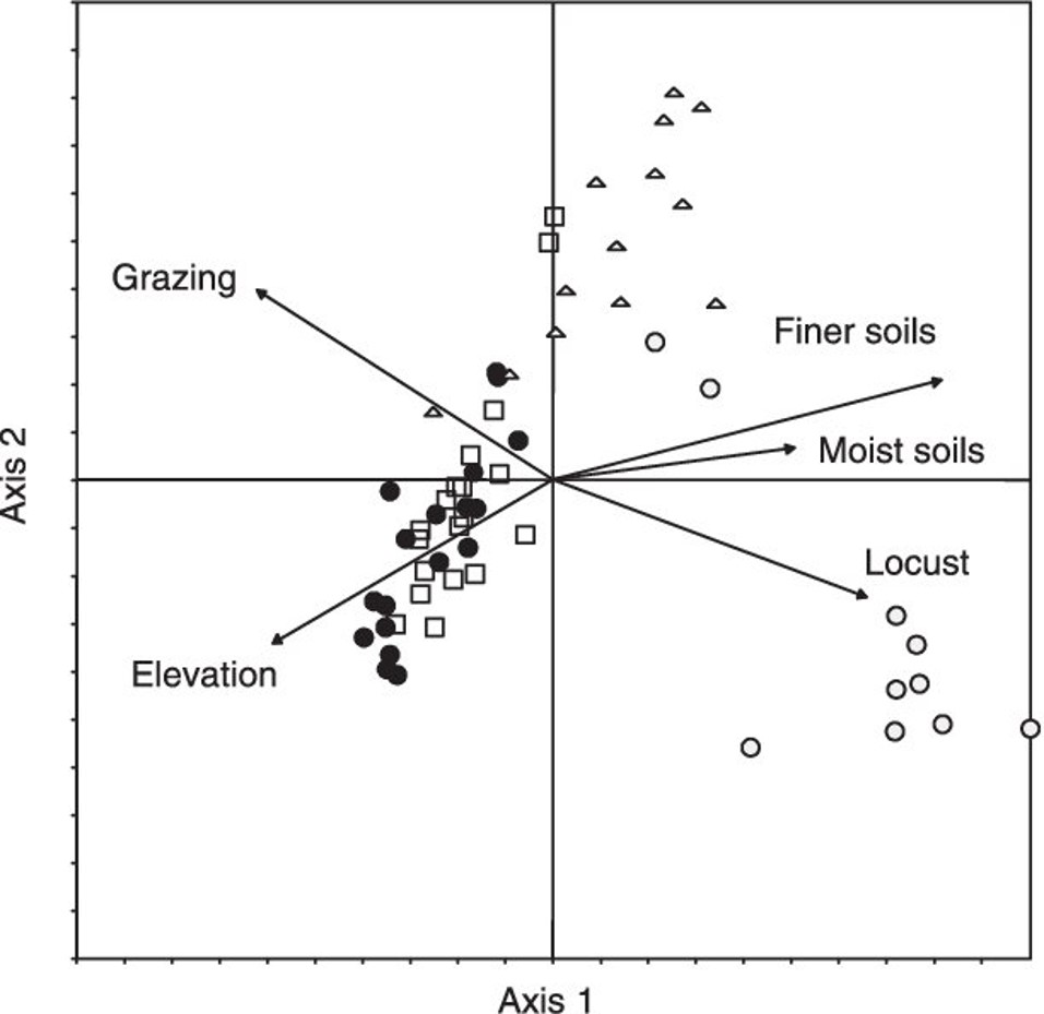
An example of a PCA ordination plot, also known as a biplot. Source: Van der Werf et al (2005) .

Another approach is to present principal components, with explained variance, in a table format and then to present linear regression analyses in separate figures. For example, Isaak et al (2018) presented the loadings of 28 temperature variables in a table format and then highlighted a correlation of the second principal component against a response variable of interest in a correlation figure.

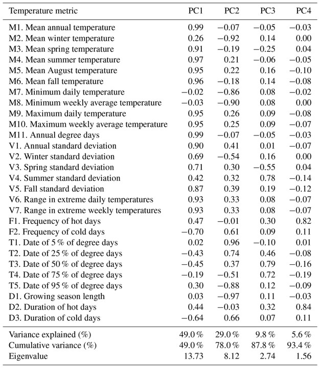
Principal components loadings can be presented in a table format with percent variance explained. Source: Table 4, Isaak et al (2018).

A principal component, or axis, can be correlated, or regressed, against the response variable. Source: Figure 10, Isaak et al (2018).

The presentation of multiple linear regression results will depend on the type of model or method that was used. For example, Forster (2012) presented data from a multiple partial linear regression analysis as a percent of variance explained in a table format:

Results from the multiple linear regression analysis can be presented in a table format. In this example, the explained variance from a partial linear regression analysis is presented. Source: Table 1, Forster (2012).

PCR in statistical packages

A PCR can be performed in the R program with a pls package: https://cran.r-project.org/web/packages/pls/index.html

Other commercially available statistical software may not explicitly offer PCR. Rather, most will offer PCA and multiple linear regression as separate procedures or modules. For these packages, a PCA on the explanatory variables will need to be performed and then a separate multiple linear regression analysis.